|
Geographic Information System (GIS) |
|
| HOME | Class Image is specially designed to handle spatial data modeling in a raster fashion. It is another way to perform Geographic Information System (GIS) operations, as oppose to vector GIS. The following are summary of built-in functions in Image that support GIS operations.
The following are some examples in GIS
|HOME| Finding suitable location for rubbish dumping area One of classical problems in GIS is to classify land with a certain set of conditions. Here we have 3 image maps, all are geo-reference. The first image map contains a natural lake, the second one shows the road network, and the last one is the land-use map. We are going to find a suitable area that is within a certain distance from the lake and the road, and it must be in a particular land-use area. First all all, we starts off with loading the lake image into an Image_uch object as follows.
It is known that all lake-pixels are having a value of 255, while the background pixels are black, zero. From it, we are going to create a distance map image where every pixel will have a value equal to the distance from the lake. It is worthwhile to mention here the distance to the lake is defined to be the shortest possible distance from the position being considered to any part of the lake. To make a distance image, we do the following.
The tif file "temp" is just for a visualization purpose, and here it is.
Next we are going to do exactly the same thing as we did before to the road network image, as follows.
Now it is the time to perform GIS operation. Suppose that we are looking for an area to make a landfill, a rubbish dumping area, we might want to locate it as far from the lake as possible, however, it should be close to the road and not in the restricted area. Noobeed processes this query in just ONE instruction away.
->best_area = Dist2road < 20 & Dist2lake > 120 & Land_use==0
Here is the result. Those pixels that are suitable for the landfill are white, while those are not are black.
The above example is somewhat a simple GIS operation, however very typical. It can be seen that the preparation step is in fact more crucial than the analysis step, and it also takes more times. More complicate analyses might need more time in the step of data preparation. For example we might have a different set of road network, where a different weight is assigned. This might lead to an additional data preparation, in which each distance map image may have to be multiplied by a different scale factor. It is up to the user imaginary and decision to create any level of complexity in GIS analysis to suite his purpose; and Noobeed is always ready for it. | HOME | Here we have a list of school location, in a text file, as follows.
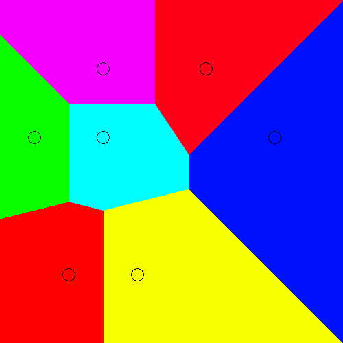
Now we are going to make a zoning map according to distance from each school location. A point that is close to a particular school must have a value of that particular school ID assigned to it. Here is a program to make a zoning map.
And here is the output image.
| HOME | |
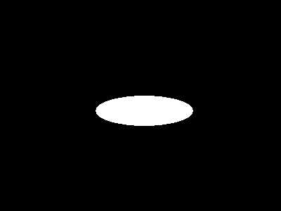 The Lake image (lake = 255, non-lake = 0)
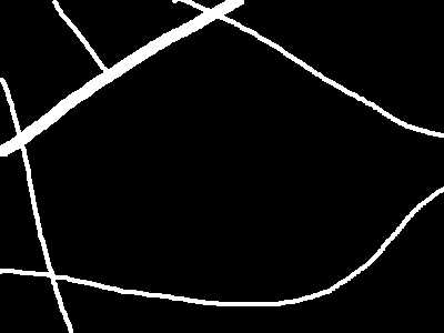 The Road image (road = 255, non-road = 0)
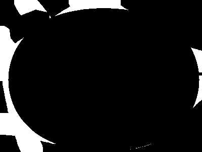
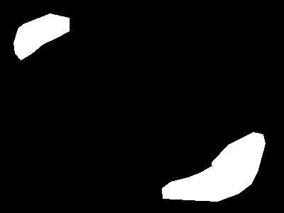 Land-use (restricted area = 255, non-restricted area = 0)
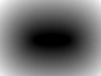 The distance map image of the lake
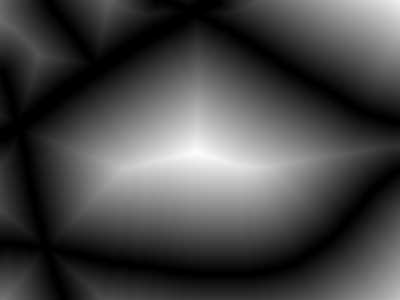 The
distance map image of the road
The
distance map image of the road