Merging Data using HSV Transformation
|
|
Merging Data using HSV Transformation |
Here we have an image of a DEM (Digital Elevation Model), we want to make a slope map and merge the slope map on top of an existing ortho-rectified image, using HSV transformation technique. In other words, we make Hue from a slope map, and we make Value, or brightness, from the ortho-photo, and combine them to make an RGB image.
Here is the DEM.
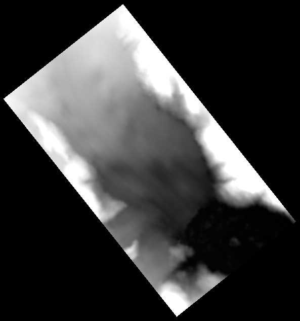
It is seen that the DEM does not cover the full extent of the image. Those background pixels have a value of -999. In Noobeed, the value of null data does not have to be always zero, like this example, zero value mean an elevation of zero meter, not a null data.
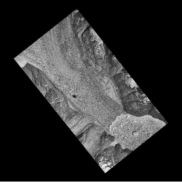
From the visualization of DEM, one might think that it is a river. In fact this is a glacier of somewhere in Greenland. Here is the ortho-rectified image of the same area.
To calculate a slope map from an DEM is actually one statement away. Here it is.
| ->A = Image_flt() | A is to store a DEM |
| ->A.load("DEM") | |
|
->B = A.slope(2)
|
this is to calculate slopes.
The value 2 of the argument means using method no 2. This method uses
8 neighboring pixels to calculate slope in x and y direction.
|
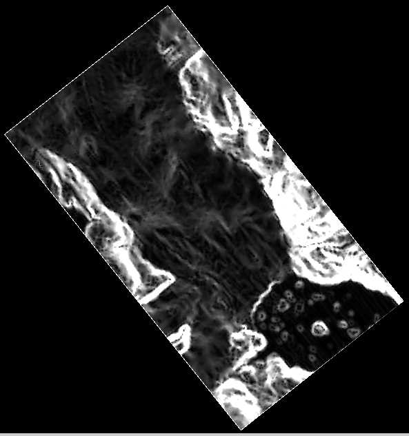
| ->B = B*100 | convert slope into percent |
| ->B.save("slope") | save slope data to file |
The result of the slope calculation is stretched and saved as a TIF file for visualization. Here it is.
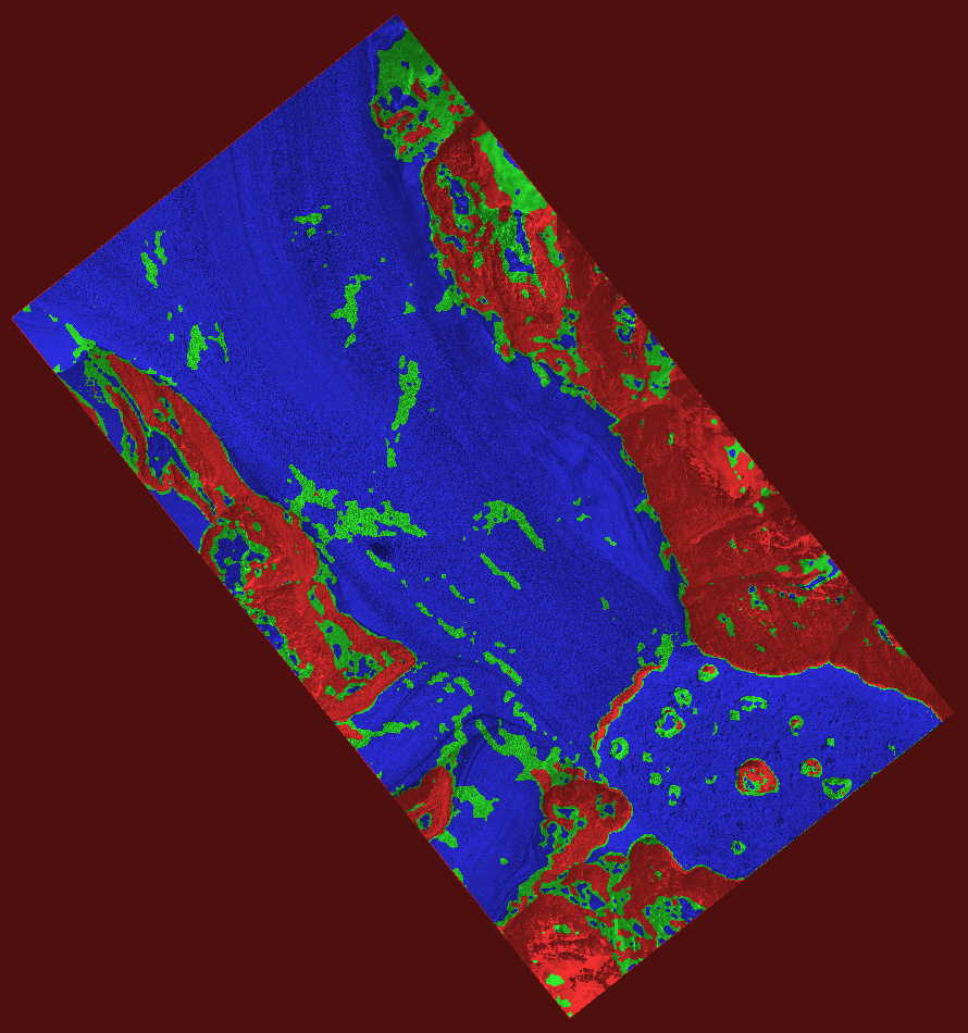
Now we are going to classify the slope values into 4 classes, then change them to HUE. Next we want to craete a saturation matrix, which is basically a constant matrix, followed by rescale the ortho-photo image to a range of 0 to 1, to make it a VALUE imahe. Finally we combine the Hue matrix, the Saturation matrix and the Value matrix to produce an RGB image. Here is the program writen in Noobeed language.
| set path "WHERE_THE_DATA_ARE" slope = image() slope.load("slope") / class 0 = < 0.0000000001 / 1 = 0.00000000001 to 5 / 2 = 5 - 10 / 3 = > 10 / class 0 is for the background data boundary = Vector(3) boundary.pushback(0.00000000001) boundary.pushback(5) boundary.pushback(10) slope_reclass = slope.reclass(boundary).uchar() hue = slope_reclass.matrix() / Hue 0 = red 120 = green 240 = blue hue.reassign(2.9,3.0,0) hue.reassign(1.9,2.0,120) hue.reassign(0.9,1.0,240)
/ stretch to a range of 0.3 to 1.0 img_rgb = Image_rgb()
|
Finally we have the result which is a combined data of an ortho-photo and its classified slope map. Slope information is represented by colors while the brightness form the image is shown as a backdrop. Here it is.