
Image rectification (Geocoding)
|
|
Image rectification (Geocoding) |
Examples in this section are:
Image rectification using classical 2D transformation
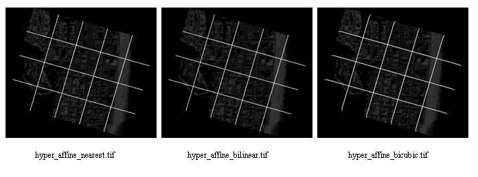
There are four types of transformations available in Noobeed, namely "conformal", "affine", "pjtive" and "poly2nd". Each of them can have three types of resample, namely "nearest", "bilinear", and "bicubic". Bilinear method uses 4 neighboring pixels for interpolation, while Bicubic interpolation requires 16 pixels.
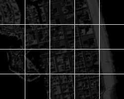
We start off with a TIF file "hyper.TIF", a hyper-spectral image (size 200 x 250). The image is intentionally made blur and a set of grid lines are added to it for a demonstration purpose.
We are going to make a collection of rectified images, using all the available transformation model and resample types. The best way is to write a small program to do the task. Here is the program.
| set path "d:\hyper" /*********** load the input TIF image fname = "hyper" A = image_uch() A.loadtif(fname) /*********** resolution of output image res = 10 /********** 4 types of Transformation tran = VecStr(4) tran.pushback("conformal") tran.pushback("affine") tran.pushback("pjtive") tran.pushback("poly2nd") /********** 3 types of Resample resamp = VecStr(3) resamp.pushback("nearest") resamp.pushback("bilinear") resamp.pushback("bicubic") /********** input image rectangular coordinate, in row and column / after read convert to X Y right hand coordinate system v1 = vecidpt2d() v1.load("img_coor") v1 = A.vidrc2xy(v1) /********** input ground control coordinate v2 = vecidpt2d() v2.load("gcp_coor") for i=0,3 for j=0,2 A_new = A.rectify(res, v1, v2, tran(i), resamp(j)) A_new.savetif(fname+"_"+tran(i)+"_"+resamp(j)) end end |
After running the program, we will have TIF files, named "hyper_conformal_nearest.tif", "hyper_conformal_bilinear.tif", ..., "hyper_poly2nd_bicubic.tif". In total there will be 16 files created, using as few as 25 lines of program codes, and finishing running in 40 seconds (Intel Pentium II 400 Mhz).
The following are some of the results of the rectified images.
Ortho-rectification of SPOT image
First we load a TIF file into a SPOT object.
->s = SPOT()
->s.loadtif("my_scene.tif")
Due to a copyright reason, the image can not be shown here. However this is just a typical TIF image file, with a size of 6000 x 6000 pixels, a panchromatic image.
Next we load two observation files, one is for image rectangular coordinates in row and column number, the other is ground control coordinate. Here they are.
->v1 = VecIdIndx()
->v1.load("obs_gcp_rc")
->v2 = VecIdPt3D()
->v2.load("obs_gcp_xyz")
It is noticed that the ground control coordinates are of the three dimensional system, as we are going to model the exterior orientation of SPOT in a rigorous mathematic model, collinearity condition. The contents of the the two observation files are as follows.
|
|
We realize that the ground control coordinates do not have a standard deviation in the file. We will assigne a reasonable value to it. Experiences suggest that an appropriate standard deviation for SPOT ground coordinates is about 3.5 meters. This applicable no matter how well the ground survey is, due to the ability to identify them on the image, which is about 0.3 pixels, or 3.5 meters.
We assigne a standrad deviation value to every point in the object "v2" by:
->v2.set_sd(3.5)
Now what we have to do is to call a class function "EO" of SPOT, as follows.
->s.EO(v1, v2, "RPT_eo")
It takes a few seconds, and the result of adjustment is stored in the file "RPT_eo.txt", as well as a set of EOPs is assigned to the SPOT object "s". The content of "RPT_eo.txt" will look like this.
| ********************************************************************************** SPOT Exterior Orientation Report(Collinearity with 1st order polynomial modelling) ********************************************************************************** SPOT image... image id : 0 no of row : 6000 no of column : 6000 focal length : 1082.000000 array length : 78.000000 array time : 9.000000 Input measure image rectangular coordinate(origin at lower left corner)... pt no x y sd 711 30.776 43.006 0.004 713 28.154 43.451 0.004 714 27.396 43.363 0.004 715 26.577 42.889 0.004 716 25.170 42.879 0.004 721 30.695 42.021 0.004 722 29.021 42.343 0.004 723 28.488 41.930 0.004 724 26.766 41.852 0.004 725 25.986 41.082 0.004 726 27.097 40.731 0.004 732 29.980 39.957 0.004 734 29.707 38.231 0.004 736 26.597 37.432 0.004 741 30.594 38.751 0.004 742 28.696 37.396 0.004 743 30.038 36.892 0.004 744 29.928 38.157 0.004 752 31.121 35.748 0.004 754 30.571 35.059 0.004 756 27.014 34.450 0.004 *** remark if sd = 0 => default sd will be used (0.060 mm) for photo coordinates ** Ground control coordinate... pt no x y z sd 711 69833.385 737233.552 649.210 3.500 713 67913.376 737876.347 638.860 3.500 714 67356.311 737898.543 647.050 3.500 715 66642.976 737644.885 657.210 3.500 716 65579.520 737806.741 635.640 3.500 721 69617.589 736495.325 615.332 3.500 722 68398.938 736937.463 622.721 3.500 723 67927.200 736696.814 626.811 3.500 724 66606.937 736855.848 614.097 3.500 725 65888.822 736352.839 638.860 3.500 726 66671.683 735960.310 613.052 3.500 732 68719.171 735037.898 615.389 3.500 734 68218.895 733768.097 628.490 3.500 736 65735.543 733539.690 665.660 3.500 741 68977.069 734048.902 634.910 3.500 742 67315.931 733246.455 635.070 3.500 743 68246.432 732718.190 630.100 3.500 744 68379.168 733682.048 628.000 3.500 752 68848.509 731711.446 610.316 3.500 754 68344.115 731260.218 617.369 3.500 756 65546.158 731253.070 629.851 3.500 *** remark if sd = 0 => default sd will be used (0.100 m)** Exterior orientation parameters... omega (deg) : 17.108990505764275 phe (deg) : -7.225817669916408 kappa (deg) : 348.713132885787620 Xo : -35690.312 Yo : 457102.646 Zo : 810253.534 dt_omega : -2.839733600792630 dt_phe : 1.492385656270120 dt_kappa : 0.471590962425169 dt_Xo : 23042.3030663170 dt_Yo : 47471.5241835071 dt_Zo : 3457.7207306428 Covariance matrix of transform parameters ... omega(sec) phe(sec) kappa(sec) Xo Yo Zo a_omega(sec) a_phe(sec) a_kappa(sec) a_Xo a_Yo a_Zo 5.225229e+008 4.183825e+008 1.946501e+007 1.679116e+009 -2.085171e+009 -2.178181e+008 -9.927705e+007 -8.731530e+007 -3.940334e+006 -3.504298e+008 3.960571e+008 4.270745e+007 4.183799e+008 3.238289e+009 2.347824e+007 1.299688e+010 -1.702329e+009 2.132436e+008 -1.719080e+008 -6.849222e+008 -5.450306e+006 -2.748974e+009 6.941214e+008 -2.362248e+007 1.946503e+007 2.347842e+007 7.272558e+006 9.423621e+007 -7.894491e+007 9.184635e+006 -7.877878e+006 -4.886086e+006 -1.579410e+006 -1.961170e+007 3.175550e+007 -9.380875e+005 1.679106e+009 1.299688e+010 9.423552e+007 5.216304e+010 -6.831913e+009 8.548732e+008 -6.897535e+008 -2.748928e+009 -2.187576e+007 -1.103298e+010 2.785032e+009 -9.470140e+007 -2.085171e+009 -1.702340e+009 -7.894484e+007 -6.831956e+009 8.325289e+009 8.214520e+008 4.075707e+008 3.553280e+008 1.606067e+007 1.426039e+009 -1.627022e+009 -1.635104e+008 -2.178177e+008 2.132447e+008 9.184655e+006 8.548776e+008 8.214503e+008 6.419704e+008 -9.119237e+007 -4.441653e+007 -2.836395e+006 -1.780559e+008 3.758060e+008 -9.837796e+007 -9.927716e+007 -1.719091e+008 -7.877878e+006 -6.897576e+008 4.075711e+008 -9.119225e+007 5.093483e+007 3.585902e+007 1.834077e+006 1.438788e+008 -2.060759e+008 1.130906e+007 -8.731474e+007 -6.849221e+008 -4.886050e+006 -2.748928e+009 3.553258e+008 -4.441630e+007 3.585880e+007 1.453815e+008 1.134840e+006 5.834949e+008 -1.447971e+008 4.857543e+006 -3.940338e+006 -5.450345e+006 -1.579410e+006 -2.187591e+007 1.606068e+007 -2.836391e+006 1.834077e+006 1.134849e+006 3.457400e+005 4.554980e+006 -7.403507e+006 3.334396e+005 -3.504276e+008 -2.748974e+009 -1.961155e+007 -1.103298e+010 1.426030e+009 -1.780550e+008 1.438780e+008 5.834949e+008 4.554947e+006 2.341883e+009 -5.809721e+008 1.947303e+007 3.960575e+008 6.941255e+008 3.175550e+007 2.785049e+009 -1.627024e+009 3.758055e+008 -2.060759e+008 -1.447980e+008 -7.403507e+006 -5.809756e+008 8.338584e+008 -4.686195e+007 4.270739e+007 -2.362259e+007 -9.380908e+005 -9.470183e+007 -1.635101e+008 -9.837797e+007 1.130908e+007 4.857565e+006 3.334403e+005 1.947312e+007 -4.686203e+007 1.532342e+007 Resiual... image rectangular coordinate gcp coordinate pt no vx vy vx vy vz 711 -0.002 0.004 1.019 1.677 -0.433 713 -0.005 -0.002 5.550 5.155 0.204 714 0.006 -0.001 -5.688 -5.777 0.109 715 -0.000 0.003 -0.214 0.283 -0.318 716 0.001 0.003 -1.112 -0.538 -0.359 721 0.004 -0.006 -2.597 -3.694 0.729 722 0.001 -0.007 0.382 -0.848 0.788 723 0.000 0.000 -0.226 -0.222 -0.000 724 -0.003 0.012 0.959 3.008 -1.328 725 -0.000 -0.010 2.162 0.450 1.082 726 -0.000 -0.005 0.935 0.029 0.575 732 -0.001 0.006 -0.204 0.895 -0.706 734 -0.001 0.006 -0.037 1.001 -0.668 736 -0.000 -0.001 0.178 0.036 0.089 741 -0.001 0.003 0.271 0.762 -0.318 742 0.002 -0.013 0.338 -1.884 1.427 743 0.001 0.009 -2.169 -0.621 -0.977 744 0.001 0.004 -2.179 -1.537 -0.393 752 -0.005 -0.007 6.501 5.329 0.695 754 0.004 -0.002 -3.701 -4.058 0.263 756 -0.001 0.004 -0.167 0.554 -0.462 no of iteration : 25 SD of unit weight : 1.699 REMARK :- ------ Stop conditions are 1. no of iterations exceeds 30 OR 2. correction to Xo, Yo, Zo coordinates are less than 0.000100 Meters ---------------------------------------------------------------- |
Please note that this example is not a good demonstration as you can see that ground control points are not well distributed over the whole image. That is why the computation took 25 iterations to convert. In fact the maximum number of iteration is redefined to 30 prior to this computation. Please also note the poor result of the covariance matrix, which is far worse than a typical result of SPOT image.
Now the SPOT object is ready to make an ortho-rectified image. We need a DEM, which must be an image object, for it has a spatial information. We will load it into an Image object, say "DEM". Then using the class function "ortho", we will be able to make an ortho-rectified image. The whole procedure takes less than 10 statements. here it is.
->resolution = 10
->s_new = s.ortho(resolution, DEM, "nearest")
Due to a copyright reason, there will be no image result shown here. We welcome if anyone would like to share the data for the presentation purpose in this area.