|
|
|

The method used here is the so-called self-calibration by bundle adjustment. It requires a test site which known ground control coordinates and a set of overlap images of the test site area, preferably 6-8 images.
The tested camera is a digital camera, Sony Cyber-shot DSC-F707. The full resolution is 1920 x 2560 pixels. However, the experiment images were taken at a resolution of 960 x 1280 pixels.
First we prepare a camera documentation file, an ordinary ASCII file. The simplest way to create it is to generate a dummy camera object, and save it using the function "save". Here it is.
->My_cam = Camera()
->My_cam.save("cam_sony")
The result
is an ASCII documentation file, where we will open to edit it. After
editing, the file looks like this.
|
Please note that fiducial marks' ID is -9. This is the way that the program recognizes a digital camera. By putting a negative ID for fiducial marks, the program knows that the camera is a digital one, and fiducial mark coordinates are interpreted as pixel sizes, and other distortion parameters. See details in class AT_BD under function "selfcalib". The pixel size in x and y direction are set to 4 micrometer, and all other distortion parameters are set to zero.
Please note that, the size of a test site may vary depending upon the application and how far the camera needed to be set from the interesting objects. The test site may be as big as several hundred meters in a traditional photogrammetry, or a couple of meters in close range photogrammetry, or as little as an A4 sheet in medication applications.
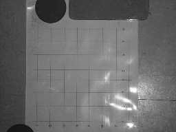
In this project we are pretending that the camera is going to take a picture of a small model, for example a teeth model in dental operation. We create a test site with the size of an A4 paper sheet consisting of 8 vertical lines and 8 horizontal lines, thus 64 points. Point coordinates are measured by an analytical plotter with an accuracy of 0.001 mm, or 1 micrometer.
Here is the image of the test site.
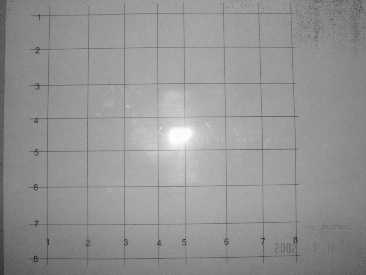
The coordinates of the 64 control points are storeed in a text file named "grid_gcp.txt".
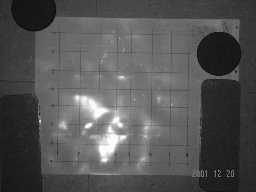
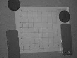
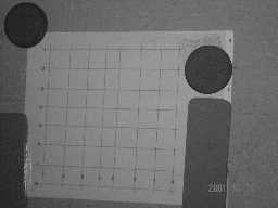
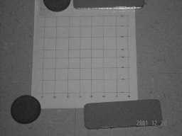
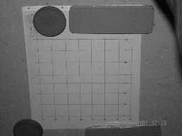
Six images of the test site are taken. The first three photos are to the left, at middle, and to the right of the test site. Then repeat again with the camera rotating at 90 degree. The left and right photos are tilted photos, while the middle one are near vertical. This is to dis-correlate the camera height with its focal length and to dis-correlate the principal point x coordinate from the y coordinate.
Here how the
6 images look.
|
"4.TIF" |
"5.TIF" |
"6.TIF" |
|
"7.TIF" |
"8.TIF" |
"9.TIF" |
Next we are going to load the 6 images, which are in "TIF" format, and perform IO and store in Noobeed format.
We wrote a
small program to process them as follows.
|
|
At this point, the relationship between x y image rectangular coordinate and xp yp coordinate is established.
Now we need to measure image rectangular coordinate of all control points in the photos. This can be done by image viewing software such as MS Paint. The observed coordinates are in fact row and column index numbers, thus conversion to xp yp coordinates are needed. The observation file containing row and column measuring data are stored in the file "obs_grid_rc.txt".
In order to convert observed row and column to xp yp photo coordinates, a program named "AT_rc2xpyp.prg" is used. See souce code and details of the program in section External Function and Program Repository. The final observation data file is stored in the file "obs_grid_xpyp.txt".
It is recommended that we first run a normal Aerial Triangulation Bundle Adjustment by using the data above. Unlike block adjustment with self calibration, regular bundle block adjustment model is more strong in the sense that the computation is almost always convert. The result from the first regular block adjustment will provide us with a set of estimation of parameters that we can use for the self-calibration adjustment later on.
Please also note that it is possible to compute a block adjustment with self-calibration right away. However there is a change that the computation gets diverged or encounters matrix rank deficiency. To prevent this happens, a set of good approximation of parameters should be used. See details in class function "selfcalib" of class "AT_BD".
So we write
a small program to do a regular block adjustment. Here it is.
|
|
We see that the standard deviation of measuring image rectangular coordinate is set to 0.005, or 5 micrometer. This is equivalent to 1 pixel on the image, since we set the pixel size to 0.004, see camera documentation file above.
The standard deviation of control point is set at 0.001, or 1 micrometer, which is the typical accuracy of an analytical plotter.
The result of the bundle block adjustment is store in a file called "adjust.rpt", with a standrad deviation of unit weight of 0.46.
Next we open
the file "adjust.rpt" and search for the adjusted parameters, the 6
EOPs, of each photo, cut it out and save in another file called
"approx.txt". Here is the file.
4 3.436670379318811e+000 3.575366204392220e+002 8.146654145334328e-001 58.291 25.642 1373.960 5 6.239472920356388e+000 3.377108595763944e+002 3.586698557718859e+002 -439.848 -33.645 1313.970 6 4.687519636474590e+000 2.034547808236986e+001 1.222314200655860e+000 627.201 22.303 1286.972 7 4.435168466168002e+000 3.545387131971148e+002 2.702557288247123e+002 1.492 -6.043 1313.089 8 2.617751034847104e+000 3.347935542541448e+002 2.700685285455387e+002 -539.000 31.322 1323.108 9 8.179750158079173e-001 3.250454762665007e+001 2.688735363921729e+002 842.900 64.912 1130.587 |
It is seen that this file has 6 lines which belong to 6 photos. Each line starts with the photo ID and followed by 6 EOPs, namely omega, phe, kappa, Xo, Yo and Zo.Now we are ready to perform Aerial Triangulation Bundle Block Adjustment with Self-Calibration. We just add a couple additional line to the previous program, as follows.
|
|
The above program sets the number of calibrated parameters to 4. They are focal length (c), xp, yp, and radial distortion parameter k1. The number of modeling calibrated parameters can be up to 9. There is no rule to how many parameters should be included in the model. The best way is to try them all, starting by a small number of parameters all the way up to the maximum number of parameters, which is 9. To do this automatically, just insert a "for loop" into the program and let the program save the results in separated files.
Theoretically, the number of parameters increase, the result standard deviation of unit weight decreases, and vice versa. However you should stop increasing the number of parameters when the standard deviation of unit weight does not change significantly.
Here is the result of the adjustment with self-calibration of the tested camera modeled by using 4 parameters, stored in the file "calib_1_4.rpt". For this particular camera, it is found that there is no significant change if more than 4 parameters are put into the calibration model.
It should be mentioned that the whole procedure for camera calibration described above is also valid for traditional aerial cameras.